Signal_Analysis.features package

Submodules

Signal_Analysis.features.signal module

Signal_Analysis.features.signal.get_F_0(signal, rate, time_step=0.0, min_pitch=75, max_pitch=600, max_num_cands=15, silence_thres=0.03, voicing_thres=0.45, octave_cost=0.01, octave_jump_cost=0.35, voiced_unvoiced_cost=0.14, accurate=False, pulse=False)

Computes median Fundamental Frequency ( \(F_0\) ). The fundamental frequency ( \(F_0\) ) of a signal is the lowest frequency, or the longest wavelength of a periodic waveform. In the context of this algorithm, \(F_0\) is calculated by segmenting a signal into frames, then for each frame the most likely candidate is chosen from the lowest possible frequencies to be \(F_0\). From all of these values, the median value is returned. More specifically, the algorithm filters out frequencies higher than the Nyquist Frequency from the signal, then segments the signal into frames of at least 3 periods of the minimum pitch. For each frame, it then calculates the normalized autocorrelation ( \(r_a\) ), or the correlation of the signal to a delayed copy of itself. \(r_a\) is calculated according to Boersma’s paper ( referenced below ), which is an improvement of previous methods. \(r_a\) is estimated by dividing the autocorrelation of the windowed signal by the autocorrelation of the window. After \(r_a\) is calculated the maxima values of \(r_a\) are found. These points correspond to the lag domain, or points in the delayed signal, where the correlation value has peaked. The higher peaks indicate a stronger correlation. These points in the lag domain suggest places of wave repetition and are the candidates for \(F_0\). The best candidate for \(F_0\) of each frame is picked by a cost function, a function that compares the cost of transitioning from the best \(F_0\) of the previous frame to all possible \(F_0's\) of the current frame. Once the path of \(F_0's\) of least cost has been determined, the median \(F_0\) of all voiced frames is returned. This algorithm is adapted from: http://www.fon.hum.uva.nl/david/ba_shs/2010/Boersma_Proceedings_1993.pdf and from: https://github.com/praat/praat/blob/master/fon/Sound_to_Pitch.cpp

Note

It has been shown that depressed and suicidal men speak with a reduced fundamental frequency range, ( described in: http://ameriquests.org/index.php/vurj/article/download/2783/1181 ) and patients responding well to depression treatment show an increase in their fundamental frequency variability ( described in : https://www.ncbi.nlm.nih.gov/pmc/articles/PMC3022333/ ). Because acoustical properties of speech are the earliest and most consistent indicators of mood disorders, early detection of fundamental frequency changes could significantly improve recovery time for disorders with psychomotor symptoms.

Parameters:

• signal (numpy.ndarray) – This is the signal \(F_0\) will be calculated from.
• rate (int) – This is the number of samples taken per second.
• time_step (float) – ( optional, default value: 0.0 ) The measurement, in seconds, of time passing between each frame. The smaller the time_step, the more overlap that will occur. If 0 is supplied the degree of oversampling will be equal to four.
• min_pitch (float) – ( optional, default value: 75 ) This is the minimum value to be returned as pitch, which cannot be less than or equal to zero.
• max_pitch (float) – ( optional, default value: 600 ) This is the maximum value to be returned as pitch, which cannot be greater than the Nyquist Frequency.
• max_num_cands (int) – ( optional, default value: 15 ) This is the maximum number of candidates to be considered for each frame, the unvoiced candidate ( i.e. \(F_0\) equal to zero ) is always considered.
• silence_thres (float) – ( optional, default value: 0.03 ) Frames that do not contain amplitudes above this threshold ( relative to the global maximum amplitude ), are probably silent.
• voicing_thres (float) – ( optional, default value: 0.45 ) This is the strength of the unvoiced candidate, relative to the maximum possible \(r_a\). To increase the number of unvoiced decisions, increase this value.
• octave_cost (float) – ( optional, default value: 0.01 per octave ) This is the degree of favouring of high-frequency candidates, relative to the maximum possible \(r_a\). This is necessary because in the case of a perfectly periodic signal, all undertones of \(F_0\) are equally strong candidates as \(F_0\) itself. To more strongly favour recruitment of high-frequency candidates, increase this value.
• octave_jump_cost (float) – ( optional, default value: 0.35 ) This is degree of disfavouring of pitch changes, relative to the maximum possible \(r_a\). To decrease the number of large frequency jumps, increase this value.
• voiced_unvoiced_cost (float) – ( optional, default value: 0.14 ) This is the degree of disfavouring of voiced/unvoiced transitions, relative to the maximum possible \(r_a\). To decrease the number of voiced/unvoiced transitions, increase this value.
• accurate (bool) – ( optional, default value: False ) If False, the window is a Hanning window with a length of \(\frac{ 3.0} {min\_pitch}\). If True, the window is a Gaussian window with a length of \(\frac{6.0}{min\_pitch}\), i.e. twice the length.
• pulse (bool) – ( optional, default value: False ) If False, the function returns a list containing only the median \(F_0\). If True, the function returns a list with all values necessary to calculate pulses. This list contains the median \(F_0\), the frequencies for each frame in a list, a list of tuples containing the beginning time of the frame, and the ending time of the frame, and the signal filtered by the Nyquist Frequency. The indicies in the second and third list correspond to each other.

Returns:

Index 0 contains the median \(F_0\) in hz. If pulse is set equal to True, indicies 1, 2, and 3 will contain: a list of all voiced periods in order, a list of tuples of the beginning and ending time of a voiced interval, with each index in the list corresponding to the previous list, and a numpy.ndarray of the signal filtered by the Nyquist Frequency. If pulse is set equal to False, or left to the default value, then the list will only contain the median \(F_0\).

Return type:

list

Raises:

• ValueError – min_pitch has to be greater than zero.
• ValueError – octave_cost isn’t in [ 0, 1 ].
• ValueError – silence_thres isn’t in [ 0, 1 ].
• ValueError – voicing_thres isn’t in [ 0, 1 ].
• ValueError – max_pitch can’t be larger than Nyquist Frequency.

Example

The example below demonstrates what different outputs this function gives, using a synthesized signal.

>>> import numpy as np
>>> from matplotlib import pyplot as plt
>>> domain = np.linspace( 0, 6, 300000 )
>>> rate = 50000
>>> y = lambda x: np.sin( 2 * np.pi * 140 * x )
>>> signal = y( domain )
>>> get_F_0( signal, rate )
[ 139.70588235294116 ]

>>> get_F_0( signal, rate, voicing_threshold = .99, accurate = True )
[ 139.70588235294116 ]

>>> w, x, y, z = get_F_0( signal, rate, pulse = True )
>>> print( w )
139.70588235294116

>>> print( x[ :5 ] )
[ 0.00715789  0.00715789  0.00715789  0.00715789  0.00715789 ]

>>> print( y[ :5 ] )
[ ( 0.002500008333361111, 0.037500125000416669 ),
( 0.012500041666805555, 0.047500158333861113 ),
( 0.022500075000249999, 0.057500191667305557 ),
( 0.032500108333694447, 0.067500225000749994 ),
( 0.042500141667138891, 0.077500258334194452 ) ]

>>> print( z[ : 5 ] )
[ 0.          0.01759207  0.0351787   0.05275443  0.07031384 ]

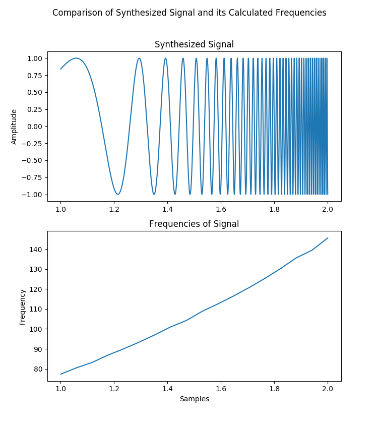
The example below demonstrates the algorithms ability to adjust for signals with dynamic frequencies, by comparing a plot of a synthesized signal with an increasing frequency, and the calculated frequencies for that signal.

>>> domain = np.linspace( 1, 2, 10000 )
>>> rate = 10000
>>> y = lambda x : np.sin( x ** 8 )
>>> signal = y( domain )
>>> median_F_0, periods, time_vals, modified_sig = get_F_0( signal,
rate, pulse = True )
>>> plt.subplot( 211 )
>>> plt.plot( domain, signal )
>>> plt.title( "Synthesized Signal" )
>>> plt.ylabel( "Amplitude" )
>>> plt.subplot( 212 )
>>> plt.plot( np.linspace( 1, 2, len( periods ) ), 1.0 / np.array(
periods ) )
>>> plt.title( "Frequencies of Signal" )
>>> plt.xlabel( "Samples" )
>>> plt.ylabel( "Frequency" )
>>> plt.suptitle( "Comparison of Synthesized Signal and it's Calculated Frequencies" )
>>> plt.show()

Signal_Analysis.features.signal.get_HNR(signal, rate, time_step=0, min_pitch=75, silence_threshold=0.1, periods_per_window=4.5)

Computes mean Harmonics-to-Noise ratio ( HNR ). The Harmonics-to-Noise ratio ( HNR ) is the ratio of the energy of a periodic signal, to the energy of the noise in the signal, expressed in dB. This value is often used as a measure of hoarseness in a person’s voice. By way of illustration, if 99% of the energy of the signal is in the periodic part and 1% of the energy is in noise, then the HNR is \(10 \cdot log_{10}( \frac{99}{1} ) = 20\). A HNR of 0 dB means there is equal energy in harmonics and in noise. The first step for HNR determination of a signal, in the context of this algorithm, is to set the maximum frequency allowable to the signal’s Nyquist Frequency. Then the signal is segmented into frames of length \(\frac{periods\_per\_window}{min\_pitch}\). Then for each frame, it calculates the normalized autocorrelation ( \(r_a\) ), or the correlation of the signal to a delayed copy of itself. \(r_a\) is calculated according to Boersma’s paper ( referenced below ). The highest peak is picked from \(r_a\). If the height of this peak is larger than the strength of the silent candidate, then the HNR for this frame is calculated from that peak. The height of the peak corresponds to the energy of the periodic part of the signal. Once the HNR value has been calculated for all voiced frames, the mean is taken from these values and returned. This algorithm is adapted from: http://www.fon.hum.uva.nl/david/ba_shs/2010/Boersma_Proceedings_1993.pdf and from: https://github.com/praat/praat/blob/master/fon/Sound_to_Harmonicity.cpp

Note

The Harmonics-to-Noise ratio of a person’s voice is strongly negatively correlated to depression severity ( described in: https://ll.mit.edu/mission/cybersec/publications/publication-files/full_papers/2012_09_09_MalyskaN_Interspeech_FP.pdf ) and can be used as an early indicator of depression, and suicide risk. After this indicator has been realized, preventative medicine can be implemented, improving recovery time or even preventing further symptoms.

Parameters:

• signal (numpy.ndarray) – This is the signal the HNR will be calculated from.
• rate (int) – This is the number of samples taken per second.
• time_step (float) – ( optional, default value: 0.0 ) This is the measurement, in seconds, of time passing between each frame. The smaller the time_step, the more overlap that will occur. If 0 is supplied, the degree of oversampling will be equal to four.
• min_pitch (float) – ( optional, default value: 75 ) This is the minimum value to be returned as pitch, which cannot be less than or equal to zero
• silence_threshold (float) – ( optional, default value: 0.1 ) Frames that do not contain amplitudes above this threshold ( relative to the global maximum amplitude ), are considered silent.
• periods_per_window (float) – ( optional, default value: 4.5 ) 4.5 is best for speech. The more periods contained per frame, the more the algorithm becomes sensitive to dynamic changes in the signal.

Returns:

The mean HNR of the signal expressed in dB.

Return type:

float

Raises:

• ValueError – min_pitch has to be greater than zero.
• ValueError – silence_threshold isn’t in [ 0, 1 ].

Example

The example below adjusts parameters of the function, using the same synthesized signal with added noise, to demonstrate the stability of the function.

>>> import numpy as np
>>> from matplotlib import pyplot as plt
>>> domain = np.linspace( 0, 6, 300000 )
>>> rate = 50000
>>> y = lambda x:( 1 + .3 * np.sin( 2 * np.pi * 140 * x ) ) * np.sin(
2 * np.pi * 140 * x )
>>> signal = y( domain ) + .2 * np.random.random( 300000 )
>>> get_HNR( signal, rate )
21.885338007330802

>>> get_HNR( signal, rate, periods_per_window = 6 )
21.866307805597849

>>> get_HNR( signal, rate, time_step = .04, periods_per_window = 6 )
21.878451649148804

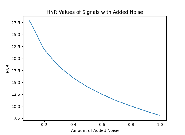
We’d expect an increase in noise to reduce HNR and similar energies in noise and harmonics to produce a HNR that approaches zero. This is demonstrated below.

>>> signals = [ y( domain ) + i / 10.0 * np.random.random( 300000 ) for
i in range( 1, 11 ) ]
>>> HNRx10 = [ get_HNR( sig, rate ) for sig in signals ]
>>> plt.plot( np.linspace( .1, 1, 10 ), HNRx10 )
>>> plt.xlabel( "Amount of Added Noise" )
>>> plt.ylabel( "HNR" )
>>> plt.title( "HNR Values of Signals with Added Noise" )
>>> plt.show()

Signal_Analysis.features.signal.get_Jitter(signal, rate, period_floor=0.0001, period_ceiling=0.02, max_period_factor=1.3)

Compute Jitter. Jitter is the measurement of random pertubations in period length. For most accurate jitter measurements, calculations are typically performed on long sustained vowels. This algorithm calculates 5 different types of jitter for all voiced intervals. Each different type of jitter describes different characteristics of the period pertubations. The 5 types of jitter calculated are absolute jitter, relative jitter, relative average perturbation ( rap ), the 5-point period pertubation quotient ( ppq5 ), and the difference of differences of periods ( ddp ).

Absolute jitter is defined as the cycle-to-cycle variation of fundamental frequency, or in other words, the average absolute difference between consecutive periods.

\[\frac{1}{N-1}\sum_{i=1}^{N-1}|T_i-T_{i-1}|\]

Relative jitter is defined as the average absolute difference between consecutive periods ( absolute jitter ), divided by the average period.

\[\frac{\frac{1}{N-1}\sum_{i=1}^{N-1}|T_i-T_{i-1}|}{\frac{1}{N}\sum_{i=1}^N T_i}\]

Relative average perturbation is defined as the average absolute difference between a period and the average of it and its two neighbors divided by the average period.

\[\frac{\frac{1}{N-1}\sum_{i=1}^{N-1}|T_i-(\frac{1}{3}\sum_{n=i-1}^{i+1}T_n)|}{\frac{1}{N}\sum_{i=1}^N T_i}\]

The 5-point period pertubation quotient is defined as the average absolute difference between a period and the average of it and its 4 closest neighbors divided by the average period.

\[\frac{\frac{1}{N-1}\sum_{i=2}^{N-2}|T_i-(\frac{1}{5}\sum_{n=i-2}^{i+2}T_n)|}{\frac{1}{N}\sum_{i=1}^N T_i}\]

The difference of differences of periods is defined as the relative mean absolute second-order difference of periods, which is equivalent to 3 times rap.

\[\frac{\frac{1}{N-2}\sum_{i=2}^{N-1}|(T_{i+1}-T_i)-(T_i-T_{i-1})|}{\frac{1}{N}\sum_{i=1}^{N}T_i}\]

After each type of jitter has been calculated the values are returned in a dictionary.

Warning

This algorithm has 4.2% relative error when compared to Praat’s values.

This algorithm is adapted from: http://www.lsi.upc.edu/~nlp/papers/far_jit_07.pdf and from: http://ac.els-cdn.com/S2212017313002788/1-s2.0-S2212017313002788-main.pdf?_tid=0c860a76-7eda-11e7-a827-00000aab0f02&acdnat=1502486243_009951b8dc70e35597f4cd19f8e05930 and from: https://github.com/praat/praat/blob/master/fon/VoiceAnalysis.cpp

Note

Significant differences can occur in jitter and shimmer measurements between different speaking styles, these differences make it possible to use jitter as a feature for speaker recognition ( referenced above ).

Parameters:

• signal (numpy.ndarray) – This is the signal the jitter will be calculated from.
• rate (int) – This is the number of samples taken per second.
• period_floor (float) – ( optional, default value: .0001 ) This is the shortest possible interval that will be used in the computation of jitter, in seconds. If an interval is shorter than this, it will be ignored in the computation of jitter ( the previous and next intervals will not be regarded as consecutive ).
• period_ceiling (float) – ( optional, default value: .02 ) This is the longest possible interval that will be used in the computation of jitter, in seconds. If an interval is longer than this, it will be ignored in the computation of jitter ( the previous and next intervals will not be regarded as consecutive ).
• max_period_factor (float) – ( optional, default value: 1.3 ) This is the largest possible difference between consecutive intervals that will be used in the computation of jitter. If the ratio of the durations of two consecutive intervals is greater than this, this pair of intervals will be ignored in the computation of jitter ( each of the intervals could still take part in the computation of jitter, in a comparison with its neighbor on the other side ).

Returns:

a dictionary with keys: ‘local’, ‘local, absolute’, ‘rap’, ‘ppq5’, and ‘ddp’. The values correspond to each type of jitter.

local jitter is expressed as a ratio of mean absolute period variation to the mean period.

local absolute jitter is given in seconds.

rap is expressed as a ratio of the mean absolute difference between a period and the mean of its 2 neighbors to the mean period.

ppq5 is expressed as a ratio of the mean absolute difference between a period and the mean of its 4 neighbors to the mean period.

ddp is expressed as a ratio of the mean absolute second-order difference to the mean period.

Return type:

dict

Example

In the example below a synthesized signal is used to demonstrate random perturbations in periods, and how get_Jitter responds.

>>> import numpy as np
>>> domain = np.linspace( 0, 6, 300000 )
>>> y = lambda x:( 1 - .3 * np.sin( 2 * np.pi * 140 * x ) ) * np.sin(
2 * np.pi * 140 * x )
>>> signal = y( domain ) + .2 * np.random.random( 300000 )
>>> rate = 50000
>>> get_Jitter( signal, rate )
{ 'ddp': 0.047411037373434134,
'local': 0.02581897560637415,
'local, absolute': 0.00018442618908563846,
'ppq5': 0.014805010237029443,
'rap': 0.015803679124478043 }

>>> get_Jitter( signal, rate, period_floor = .001,
period_ceiling = .01, max_period_factor = 1.05 )
{ 'ddp': 0.03264516540374475,
'local': 0.019927260366800197,
'local, absolute': 0.00014233584195389132,
'ppq5': 0.011472274162612033,
'rap': 0.01088172180124825 }

>>> y = lambda x:( 1 - .3 * np.sin( 2 * np.pi * 140 * x ) ) * np.sin(
2 * np.pi * 140 * x )
>>> signal = y( domain )
>>> get_Jitter( signal, rate )
{ 'ddp': 0.0015827628114371581,
'local': 0.00079043477724730755,
'local, absolute': 5.6459437833161522e-06,
'ppq5': 0.00063462518488944565,
'rap': 0.00052758760381238598 }

Signal_Analysis.features.signal.get_Pulses(signal, rate, min_pitch=75, max_pitch=600, include_max=False, include_min=True)

Computes glottal pulses of a signal. This algorithm relies on the voiced/unvoiced decisions and fundamental frequencies, calculated for each voiced frame by get_F_0. For every voiced interval, a list of points is created by finding the initial point \(t_1\), which is the absolute extremum ( or the maximum/minimum, depending on your include_max and include_min parameters ) of the amplitude of the sound in the interval \([\ t_{mid} - \frac{T_0}{2},\ t_{mid} + \frac{T_0}{2}\ ]\), where \(t_{mid}\) is the midpoint of the interval, and \(T_0\) is the period at \(t_{mid}\), as can be linearly interpolated from the periods acquired from get_F_0. From this point, the algorithm searches for points \(t_i\) to the left until we reach the left edge of the interval. These points are the absolute extrema ( or the maxima/minima ) in the interval \([\ t_{i-1} - 1.25 \cdot T_{i-1},\ t_{i-1} - 0.8 \cdot T_{i-1}\ ]\), with \(t_{i-1}\) being the last found point, and \(T_{i-1}\) the period at this point. The same is done to the right of \(t_1\). The points are returned in consecutive order. This algorithm is adapted from: https://pdfs.semanticscholar.org/16d5/980ba1cf168d5782379692517250e80f0082.pdf and from: https://github.com/praat/praat/blob/master/fon/Sound_to_PointProcess.cpp

Note

This algorithm is a helper function for the jitter algorithm, that returns a list of points in the time domain corresponding to minima or maxima of the signal. These minima or maxima are the sequence of glottal closures in vocal-fold vibration. The distance between consecutive pulses is defined as the wavelength of the signal at this interval, which can be used to later calculate jitter.

Parameters:

• signal (numpy.ndarray) – This is the signal the glottal pulses will be calculated from.
• rate (int) – This is the number of samples taken per second.
• min_pitch (float) – ( optional, default value: 75 ) This is the minimum value to be returned as pitch, which cannot be less than or equal to zero
• max_pitch (float) – ( optional, default value: 600 ) This is the maximum value to be returned as pitch, which cannot be greater than Nyquist Frequency
• include_max (bool) – ( optional, default value: False ) This determines if maxima values will be used when calculating pulses
• include_min (bool) – ( optional, default value: True ) This determines if minima values will be used when calculating pulses

Returns:

This is an array of points in a time series that correspond to the signal’s periodicity.

Return type:

numpy.ndarray

Raises:

ValueError – include_min and include_max can’t both be False

Example

Pulses are calculated for a synthesized signal, and the variation in time between each pulse is shown.

>>> import numpy as np
>>> from matplotlib import pyplot as plt
>>> domain = np.linspace( 0, 6, 300000 )
>>> y = lambda x:( 1 + .3 * np.sin( 2 * np.pi * 140 * x ) ) * np.sin(
2 * np.pi * 140 * x )
>>> signal = y( domain ) + .2 * np.random.random( 300000 )
>>> rate = 50000
>>> p = get_Pulses( signal, rate )
>>> print( p[ :5 ] )
[ 0.00542001  0.01236002  0.01946004  0.02702005  0.03402006 ]

>>> print( np.diff( p[ :6 ] ) )
[ 0.00694001  0.00710001  0.00756001  0.00700001  0.00712001 ]

>>> p = get_Pulses( signal, rate, include_max = True )
>>> print( p[ :5 ] )
[ 0.00886002  0.01608003  0.02340004  0.03038006  0.03732007 ]

>>> print( np.diff( p[ :6 ] ) )
[ 0.00722001  0.00732001  0.00698001  0.00694001  0.00734001 ]

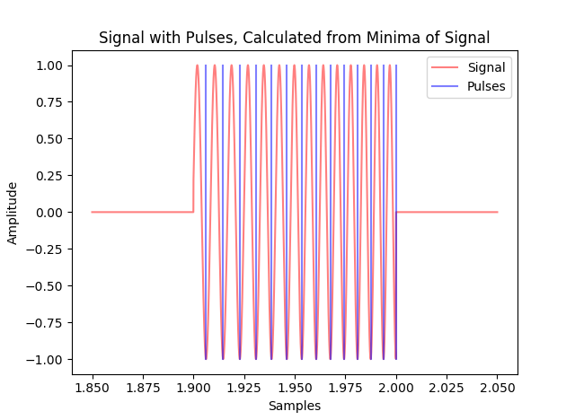
A synthesized signal, with an increasing frequency, and the calculated pulses of that signal are plotted together to demonstrate the algorithms ability to adapt to dynamic pulses.

>>> domain = np.linspace( 1.85, 2.05, 10000 )
>>> rate = 50000
>>> y = lambda x : np.sin( x ** 8 )
>>> signal = np.hstack( ( np.zeros( 2500 ), y( domain[ 2500: -2500 ] ),
np.zeros( 2500 ) ) )
>>> pulses = get_Pulses( signal, rate )
>>> plt.plot( domain, signal, 'r', alpha = .5, label = "Signal" )
>>> plt.plot( ( 1.85 + pulses[ 0 ] ) * np.ones ( 5 ),
np.linspace( -1, 1, 5 ), 'b', alpha = .5, label = "Pulses" )
>>> plt.legend()
>>> for pulse in pulses[ 1: ]:
>>>     plt.plot( ( 1.85 + pulse ) * np.ones ( 5 ),
np.linspace( -1, 1, 5 ), 'b', alpha = .5 )
>>> plt.xlabel( "Samples" )
>>> plt.ylabel( "Amplitude" )
>>> plt.title( "Signal with Pulses, Calculated from Minima of Signal" )
>>> plt.show()

Module contents